Music Technology

+ Expand All

Research - GPU Acceleration of Real-time Reverberation

Summary

This was my master's thesis at NYU. I essentially benchmarked raytracing on a CPU and a GPU, using pyroomacoustics and OptiX 7.0. For a certain configuration, a Pascal series P100 chip performed 396x faster than the CPU implementation.

Check it out on GitHub!

Email me if you'd like to see the full document.

Defense Video

Jefferson Refresh

Summary

Look down below at the heading "Binaural Spatializer in OpenGL/CUDA(v 1.5 - Jefferson)" for introductory details regarding Jefferson. With the help of Vinny Huwyn, Jefferson got a facelift. I also implemented frequency domain HRTF interpolation and ASSIMP for easier model imports.

Check it out on GitHub

Paper

Research - GPU Acceleration of Massive Convolution

Introduction/Description

GPU Acceleration of Massive Convolution - aka: How long will it take to add reverb to all of Avengers: Endgame?

If you're not familiar with the term reverb, it's what you hear when you clap in a bathroom or a church. It’s an audio effect that can make a recording sound like it’s in a church or in a small room. Apply it to an audio track and now your singer sounds like they’re in a huge concert hall. There are two mathematical ways to apply reverb to an audio track, and the one I’m focusing on is called convolution.

It’s got a long, technical name, but convolution reverb sounds the best. It requires an impulse response of a room and the signal you want to add reverb to. An impulse response is a recording of a room. The easiest way to do it is to pop a balloon or clap (very loudly!). The bigger the room, the longer the reverb trail will be. This recording contains all of the sonic features of the room.

The intuitive way to apply this impulse response is to shape every single sample of your input with the reverb. Meaning, take the first sample of your signal and multiply it by every single sample of the reverb.

Visual representation of convolution 1

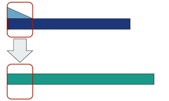
This emulates a reverb trail for the first sample. Then, continue this for every single sample of the input. The reverb trails overlap with each other, so they are added together.

Visual representation of convolution 2

The overlapping reverb trails is like trying to talk in a gymnasium. If too many people talk at once, the echoes overlap with each other and you can't hear what the other person is saying.

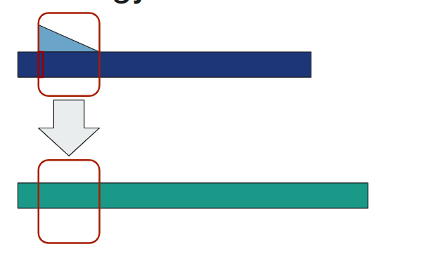
Another way to think about this is that a single sample of the output is the sum of all the echoes in a given moment in time.

Visual representation of convolution 3

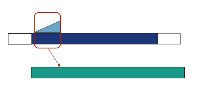
The math checks out, and both algorithms do the same thing since order doesn’t matter with multiplication and addition. This second way is used more often in digital signal processing because it has a formula:

Discrete Convolution Formula

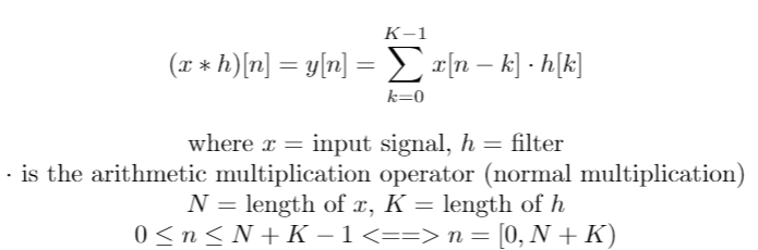
When we tell a computer to use this formula to come up with reverb, the computer doesn’t really like it. That’s because this method involves a huge amount of addition and multiplication operations. The actual number of computations is N * K, which grows to N^2 if the reverb is the same length as the input.

Ok, here’s a real-world analogy. Avenger’s: Engame is 3 hours long, or 180 minutes. At a standard 48kHz sample rate, that’s 518.4 million samples. If we wanted to add a 10 second reverb to the entire movie, the reverb would be 480 thousand samples. That means 518.4 million x 480 thousand = 248.8 trillion number of operations. A standard CPU from 2014 (Intel i5-557R) can do up to 179.2 million operations per second. Theoretically, it would take 1,388,571 seconds = 23,142 minutes = 385 days = 1 year and 21 days to compute.

Ouch!

There is another way to do this using the Fast Fourier Transform and going into the frequency domain. I won’t go into details, but it’s significantly faster with a theoretical estimate of 263 seconds = 4.4 minutes. I call these two methods time domain convolution and frequency domain convolution. That's a lot better than a year, but we can do better.

This is where the GPU comes in. A GPU also released in 2014 has a theoretical peak of 6840 million operations per second. Following the same math, it would take 10 hours using time domain convolution and 6.9 seconds using the frequency domain convolution.

That sounds so much better!

The problem with these estimates is that they are impossible to reach due to physical constraints. A computer consists of multiple parts, some of which are slower than others. The CPU needs to talk to the memory to get the numbers to do the computations, and the memory is over 100x slower than the CPU.

The only way to truly find out how long it takes is through experimentation. That’s exactly what I did.

Background Knowledge and Tools

FFTW3 - short for Fastest Fourier Transform in the West. It is an FFT library in C/C++
FFTW Main Page
FFTW Documentation

CUDA - acronym for Compute Unified Device Architecture. It’s “a parallel computing platform and programming model developed by NVIDIA for general computing on graphical processing units (GPUs)” (Nvidia). It is a proprietary but free API in several different programming languages to speak directly to NVIDIA hardware and utilize parallel processing.
General Knowledge
Download link
Documentation

cuFFT – NVIDIA CUDA Fast Fourier Transform library.
General knowledge
Documentation

Thrust – “Thrust is a C++ template library for CUDA based on the Standard Template Library (STL)” (Nvidia). It’s a library within CUDA that utilizes parallel processing for algorithms that already exist in C++’s standard library such as summing, reducing, and sorting.
NVIDIA Documentation
GitHub Documentation

Libsndfile – Portable audio library used to read contents of wave files
Download link

Credits to Dr. Brian McFee for the DSP knowledge and Dr. Mohamed Zahran for the GPU knowledge.

Source Code

Research Paper

Conclusions

For time domain convolution, the GPU is slower than the CPU until the input size reaches 2 10. This is 1024 samples, or 10 milliseconds of audio at 96kHz. 228 samples, the highest test value for both, is just over a quarter of a billion samples, or about 46 minutes of audio at 96kHz. This number of samples on a CPU took 4 days, 18 hours, and about 27 minutes to compute, while it took 13 minutes on the GPU. That's a ~50x speedup. It's also incredibly unreasonable to wait 4 days to process a single audio file. As started earlier, considering that the time approximately doubles for each doubling of input size, 2 29 is projected to take 9 days, and 230 is projected to take 19 days.

For frequency domain convolution, the GPU begins to be useful for inputs of 2 23and above. This is equivalent to 8,388,608 samples or ~87 seconds of audio at 96kHz. At 230 samples, which is just over 1 billion samples or just over 3 hours of audio, there is a ~44x speedup from ~8.7 minutes to ~11.8 seconds.

Combining these these results, CPU frequency domain convolution is the fastest for inputs smaller than 223 samples (~87 seconds), and GPU frequency domain convolution is the fastest for any inputs larger than that.

Binaural Spatializer in OpenGL/CUDA(v 1.5 - Jefferson)

Summary

I’ve been working on this project since April 2018, and it is meant to explore CUDA, OpenGL, and Binaural audio.

The cartoon character represents the listener, and the green sphere represents the sound source. The user can use arrow keys to move the sound source up, down, forwards, backwards, left, and right throughout the 3D space, and the audio will adjust to sound like it’s coming from that direction and distance. The user can also use the mouse to rotate the viewing angle and zoom in/out.

Background Knowledge and Tools

OpenGL - short for Open Graphics Library. It is an API/library in several programming languages to draw 2D and 3D images. It’s portable and it’s implemented primarily in each computer’s hardware.

CUDA - acronym for Compute Unified Device Architecture. It’s “a parallel computing platform and programming model developed by NVIDIA for general computing on graphical processing units (GPUs)” (Nvidia). It is a proprietary but free API in several different programming languages to speak directly to NVIDIA hardware and utilize parallel processing.
General Knowledge
Download link
Documentation

cuFFT – NVIDIA CUDA Fast Fourier Transform library.
General knowledge
Documentation

Thrust – “Thrust is a C++ template library for CUDA based on the Standard Template Library (STL)” (Nvidia). It’s a library within CUDA that utilizes parallel processing for algorithms that already exist in C++’s standard library such as summing, reducing, and sorting.
NVIDIA Documentation
GitHub Documentation

HRTF – acronym for Head Related Transfer Function. Several short audio filters depending on angle (azimuth) and elevation that can make a sound come from different locations in 3D space. The ones I used were the compact set from MIT and KEMAR

PortAudio - Portable audio library used to connect to the computer’s sound device
Download link

Libsndfile – Portable audio library used to read contents of wave files
Download link

Blender – Open source, free 3D creation suite
Download link

3ds – 3D Model file type importable/exportable by blender. I used Damiano Vitulli’s code to import 3ds files into my OpenGL program.

Technical Description

This project uses OpenGL to create a 3D visualization of two objects in space and then convolves audio using an HRTF to match the distance and angle of the two objects. It also utilizes parallel processing and the speed of a GPU. The project’s original purpose was to experiment with parallel processing and to see if CUDA can speed up real-time convolution, which I have not been able to solve yet. However, this result can be useful for VR/AR audio and being able to record audio whose source is being moved in 3D space.

Using libsndfile, this project takes in a 44.1k sample rate input file and reverb impulse response. If the input file is stereo, it is summed to mono using the formula R[i] = (L[i] + R[i]) / 2. If the reverb file is in stereo, the program terminates. Using cuFFT, it does convolution reverberation on the input file, and then stores that data into a buffer in the RAM and onto the disk as a file. I used thrust to calculate the RMS of both signals. Then, the program reads and stores 366 different HRTF impulse responses at various elevations and azimuths. The audio starts playing through PortAudio, and the graphical interface is then displayed to affect what is played.

A purple cartoon character indicates the listener, which remains in the same spot in the middle. The green indicates the sound source. Different keys listed below will move the sound source in the X, Y, and Z axes. The visualization can also be rotated by left clicking and dragging the visualization which helps to better visualize the 3D space. The user can also zoom in and out by clicking and dragging the right arrow key or by using the scroll wheel. The R key will reset back to the default perspective and position. My program also optionally writes the output to a sound file.

The standard orientation in OpenGL looks like this:

OpenGL Axis Orientation

This is how I mapped the keys to be more visually intuitive:

Key Result
UP -Z
DOWN +Z
LEFT / A -X
RIGHT / D +X
W +Y
S -Y
Left click & drag Rotate
Scroll wheel / right click & drag Zoom in/out

In version 1.5, I added a cartoon character named Jefferson and modified the locations of the sound source and listener to be more intuitive.

The cartoon character, which I’ve fondly named Jefferson, is available here as a free download. I also used this person’s bowler hat model. The letter J was created in Microsoft’s Paint 3D. I used Blender to combine, resize, scale, and export the character’s parts to a 3ds file, which I then imported into my program. Here’s what it looks like in Blender:

Future Plans

My next plan is to include a moving visualization of the waveform that will travel from the sound source to Jefferson. After that, I would like to enhance the HRTF and audio quality.

Tap Tempo Guitar Pedal (Fall 2017)

Guitar Pedal Image 1 Guitar Pedal Image 2

This was a guitar pedal made out of cardboard for my analog electronics class. The bottom panel has 4 buttons, each for a different setting. The settings are bypassed signal, soft clipping distortion, hard clipping distortion, and what I call a sweeper. A sweeper is similar to a wah pedal with slightly different circuitry. The switch next to the red buttons does something a bit weird – it cycles through all 4 settings, and the “tempo” of the switching is controlled through one of the knobs.

On the top panel, there’s a gain control knob and a knob to control the frequency of the sweeper. The two switches allow for hard or soft clipping respectively and sweeping. The button is a tap tempo button to establish the tempo of the cycling, and the last knob is for tone control.

The project overall isn't as rugged as I would like it to be - especially because the prototype was built in one day and is completely made out of cardboard. I'm satisfied with it right now, because I'm not sure what to do with it, however I may use a 3D printer and create a better, sturdier, more user-friendly casing and interface.
Click here for more technical details!

Staple Remover Keyboard Pedal (Summer 2016)

In the end of my freshman year, my friend Jake Sandakly just got a new MIDI keyboard and we were playing with it. I said I wish we had a sustain pedal. Then I made promise to him that I would build him a sustain pedal. I'm sure he thought I was just joking. I was at work at my job for IT that summer, idly zoning out for a few moments, and I was blankly staring at a staple remover. Then I realized that the staple remover has the perfect spring action required for a pedal, and it'll always pop back up. I built a prototype from cardboard that fell apart. Then, I went back home to Rochester in August and started cutting wood to glue onto this staple remover. I stripped some broken headphones for the jack, got some paperclips, soldered everything together, and successfully built it. It's extremely fragile still, and it is so light that it keeps getting pushed back whenever it's pressed, but it works. This project is also still in process... mainly because it broke in transit from Rochester to New York to Grafton, MA, and back to New York.

Shoe Drum Machine (Spring 2016)

Shoe Drum Machine image 1 Shoe Drum Machine image 2

I was playing some rock songs on the piano in college, then I got to the point where I really wished I could play a drumset at the same time. Throughout the winter on the bus, in class, on the subway, I’d sit idly and pretend that I was playing drums with my feet. I’d pretend the heels of my boots were bass drums and the ball of my foot was a snare drum. Then I thought – “What if I combined this with piano?”

A few months later, this became my final project for my Digital Electronics class. I have shoes with force sensitive resistors in the heels of both shoes and one in the ball of my left foot. The harder I stomp, the louder the drum sound will be. This is connected to a control panel with a touchpad of 16 numbers, 6 knobs, and a ribbon potentiometer. The touchpad had standard drumbeats built-in from number 2-12. Number 1 was a tap-tempo for these preset drumbeats. Number 13, 14, and 15 would trigger random drumfills at 8th notes, triplets, or 16th notes respectively. Number 16 stopped the preset drumbeat. These could be played in conjunction with the shoes. The knobs changed the velocity values for the various drum sounds in the preset drums. Lastly, the ribbon potentiometer could emulate a suspended cymbal roll when I drag my finger across it.

This project is by no means perfect, and the item I currently have is a prototype. It’s functional for now even though it’s very fragile, and I plan on improving it in various ways. For instance, I’d like to use OOP to condense the code and a 3D printer to create a better control panel. I could also use different sensors – the ribbon potentiometer isn’t sensitive enough, and the touchpad is far too sensitive.
Click here for more technical details!